Getting the Right Exposure for Good Point Clouds
Introduction
The method described in this section is aimed at capturing a complete point cloud of the entire scene. In many real applications, it is only necessary to get a good exposure of certain objects or regions within the scene. The same method can be applied in those scenarios, but regions that are not of interest do not need to be exposed.
In this tutorial, we will use the histogram function in Zivid Studio to help us assess the quality of the point cloud as we find our exposure values. The goal is to expose as many pixels as possible with sufficiently high SNR so that the point cloud gets low temporal noise.
In Zivid Studio, the SNR can be seen in the 2D RGB or depth map image. Hover the mouse cursor over a pixel, and the SNR for that pixel will be visible in the bottom left corner of the screen, as shown here. An SNR value of 7 and above is considered good. Such SNR values typically relate to the RGB channels being exposed well, with a value between 32 and 255. The method in this article aims to cover as many pixels as possible within this region.
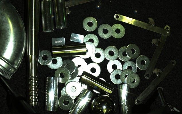
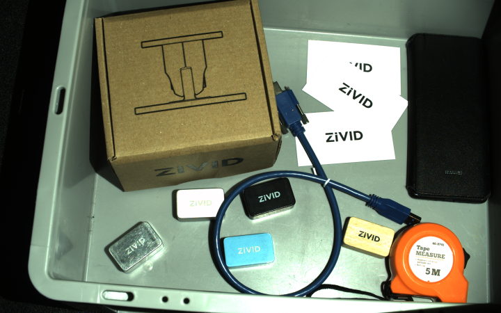
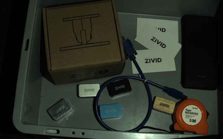
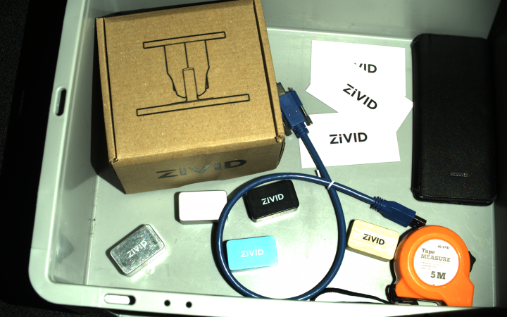
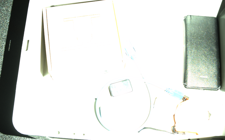
This tutorial assumes that the scene includes both very shiny materials, such as metal cylinders, and dark materials, such as black plastics. It also assumes that imaging occurs in an environment exposed to ambient light powered by power lines of 50 Hz frequency. An example scene is shown in the image below.
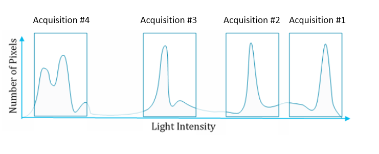
Such scenes may contain a significantly wider dynamic range than the Zivid 3D cameras can capture within a single acquisition. Hence it is often required to use Zivid’s HDR function with multiple acquisitions for different regions of the intensity spectrum, as illustrated in the image below.
Note
The Zivid Two uses 12-bit images and thus covers a higher dynamic range than the Zivid One+ with single acquisitions. Hence, with Zivid Two, it is possible to cover the same dynamic range with fewer acquisitions.
Note
Single acquisitions using Stripe Engine cover a wider dynamic range than single acquisitions using Phase Engine. Stripe Engine’s dynamic range benefit is more noticeable for Zivid One+ cameras. It is not that noticeable for Zivid Two because the Phase Engine with Zivid Two covers a wider dynamic range than the Phase Engine with Zivid One+. The Stripe Engine provides more benefits than just covering a wider dynamic range such as dealing with reflections.
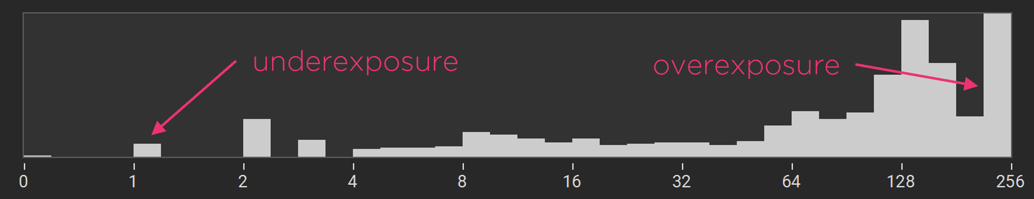
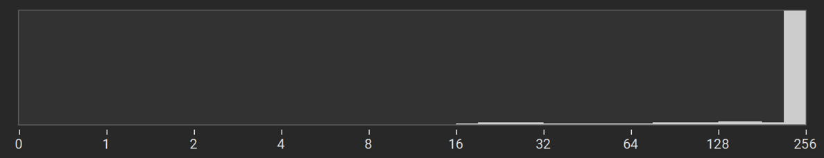
The histogram
The histogram in Zivid Studio is a powerful tool for evaluating point cloud quality. It counts how many pixels have a distinct intensity value within an image and displays them in bins from 0 to 255. The histogram method that we use to evaluate point cloud quality is based on a relationship between the pixel intensity and its 3D quality. The higher the pixel intensity (unless saturated), the higher the SNR, thus higher the 3D quality. Each bin represents one exposure stop when displaying the histogram with a logarithmic x-axis. This representation makes it very convenient to estimate which exposure values are needed to expose certain regions of the scene well.
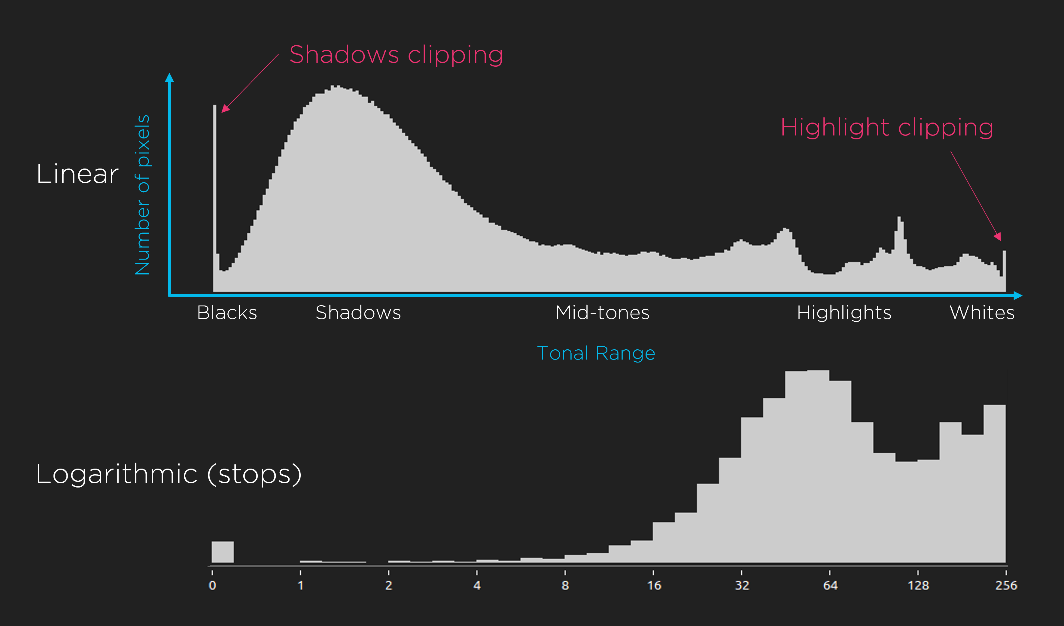
The image above shows an example of a histogram where the scene is well exposed. We can tell this because most of the pixels are in the upper right half of the logarithmic graph. The following is also easy to see from the histogram. Doubling the intensity, or adding one exposure stop, will “move” the hump formed by pixels with intensity from 64 to 128 to the right-most area of the histogram. We can achieve this, for example, by doubling the exposure time.
Caution
The default Color Mode is Automatic, which is identical to ToneMapping for multi-acquisition HDR captures with differing acquisition settings. Tone mapping modifies pixel values and thus affects the histogram, making it impossible to use the histogram to evaluate exposure quality. Therefore, when using the histogram, you must evaluate one acquisition at a time and set the Color Mode to UseFirstAcquisition or Automatic.
Caution
Gamma correction and Color Balance setting modifies pixel values and thus making it impossible to use the histogram to evaluate exposure quality. Therefore, you must set Gamma and Color Balance to 1.0 when using the histogram.
Introduction to the Stops Table
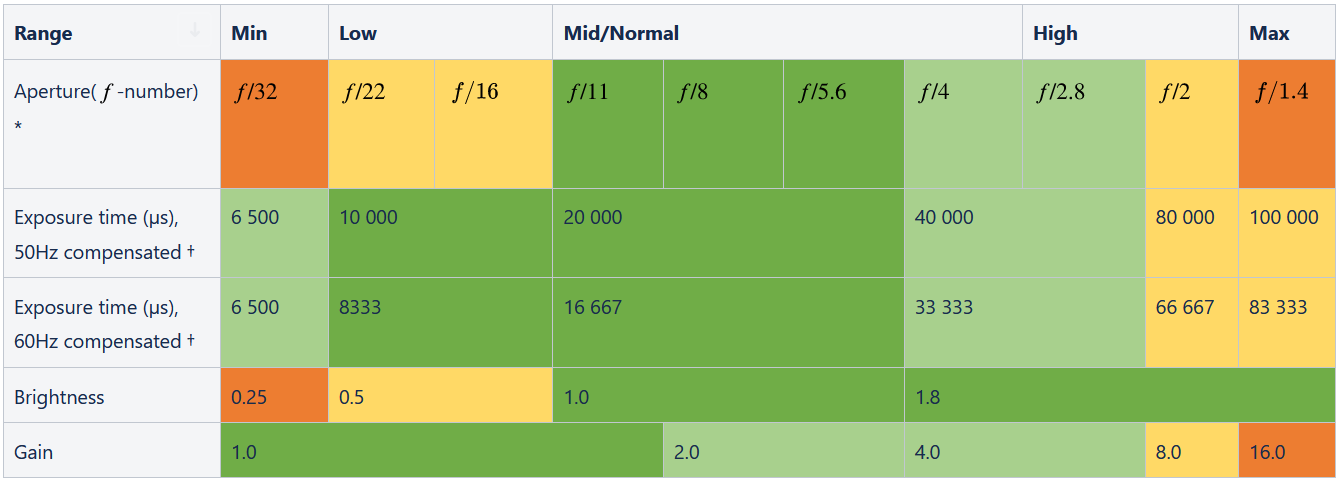
A second powerful tool that we will use is the Stops Table. The table shows the span of the Zivid 3D cameras’ stops, where each row shows the available range for each of the exposure parameters in Zivid. Each cell represents a stop position for one of the four exposure variables in the Zivid camera: aperture, exposure time, brightness and gain. To increase exposure with one stop, we move one cell to the right for a specific variable. To decrease exposure with one stop, we move one cell to the left for a specific variable. Example: the current exposure time is 10 000 μs. We want to increase the exposure with one stop. We increase the exposure time to 20 000 μs.
Note that the table shows two rows for exposure time. Use the correct row to compensate for 50 Hz or 60 Hz power-line frequency as described in the Exposure Time. The Stops Table is created for Zivid One+. Values vary for Zivid Two; see below.
Note
The color-coding of the cells shows how “good” the values are. The strong green color is considered a highly recommended value to use. Light green cells are also considered good, while yellow cells are not considered very good to use. Red columns should be avoided unless necessary. Thus, exposure values should be composed of parameter values in green cells as much as possible.
Tip
Try to build your exposure values with combinations of green cells from the stops table.
Note
The values of certain exposure settings can affect the quality of the color image. Considerations to take for good color image quality are covered later in Adjusting Acquisition Settings section in Optimizing Color Image.
Preparation - relaxing filters
To evaluate as many good points as possible, we start by relaxing all filters. After finding all exposure values, set the filters as the last step. We relax the filters by setting the following filter values:
Noise: 1.0
Gaussian: Disabled
Reflection: Disabled
Outlier: 50
Contrast Distortion: Disabled
Hole Filling: Disabled
Acquisition #1 - exposing for highlights
We want to start by exposing the highlights and then gradually increase our exposure to include mid-tones and eventually lowlights (dark regions). If the following procedure is insufficient to achieve good data on especially shiny and bright parts, we recommend that you follow the steps in Dealing with Highlights and Shiny Objects as your first acquisition.
Step 1 - set low exposure values
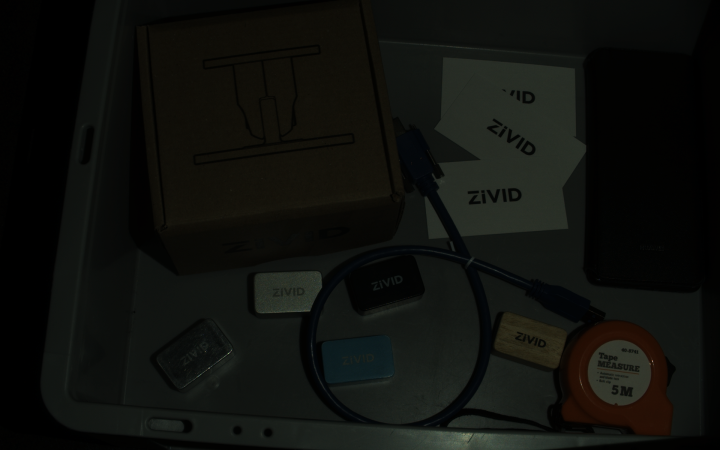
We begin by turning off all but one acquisition, so we only have a single acquisition capture. Then, we set our exposure very low so that no pixels in the image (or the histogram) have an RGB value of 255. The following starting condition should work on most occasions.
Aperture (\(f\)-number): 32
Exposure time: 10 000 (8 333 in regions with 60 Hz power line frequency)
Brightness: 1.0
Gain 1.0
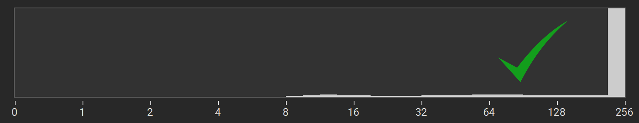
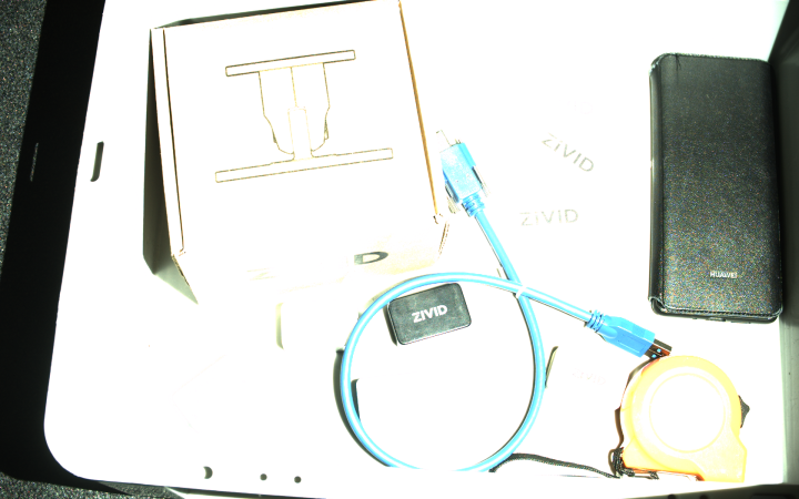
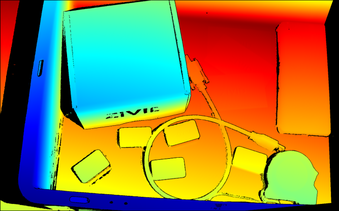
If there are still regions in the image that are overexposed, as illustrated in the figure above, try to reduce the exposure time further and increase the \(f\)-number. The figure below shows a capture with no overexposed pixels.
Step 2 - get good exposure on brightest pixels
Decrease the \(f\)-number by moving one stop in the Stops Table at a time to the right. Carry this out until the brightest pixels have an intensity close to 255. Verify that the highlights in your scene have data by observing the point cloud or the RGB image. The highlight regions are typically on edges or on top of spheres and cylinders of shiny objects.
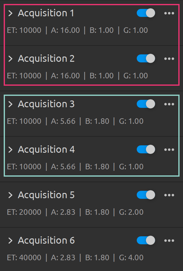
In our example, we would need to increase by two stops. Our first acquisition would, therefore, consist of the following values:
Aperture (\(f\)-number): 16
Exposure time: 10 000 (8 333 in regions with 60 Hz power line frequency)
Brightness: 1.0
Gain 1.0
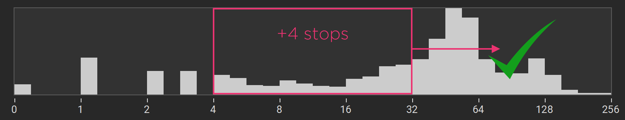
Acquisition #2 - exposing for mid-tones
After covering the highlights, we want to move on to exposing more of the image. By looking at the histogram, we identify the next portion of the image exposed with an intensity below 32. We want to move this region up in the upper half of the image towards 255, typically done by adding three-four stops. Adding the first stop by maximizing projector brightness is typical because it gives the highest possible SNR. Then we want to add three more stops by increasing the aperture to use aperture values that reside in green cells.
Step 1 - new acquisition
Add another acquisition and disable the first acquisition.
Step 2 - increase exposure
Move a total of three or four more stops to the right. The first stop should be maximizing brightness, and the other stops should typically come from the aperture.
The example, acquisition #1 from above has an aperture of 16. Therefore, move three aperture stops to the right (count aperture columns in the Stops Table), which results in aperture 5.6. Finally, increase the projector brightness from 1.0 to 1.8.
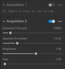
Acquisition #2 will then have the following values:
Aperture (\(f\)-number): 5.6
Exposure time: 10 000 (8 333 in regions with 60 Hz power line frequency)
Brightness: 1.8
Gain: 1.0
Acquisition #N - keep increasing exposure towards lowlights
Repeat the procedure for acquisition #2. Locate the next region of pixels that needs to be exposed higher and count the number of stops required to bring the intensity of those pixels close to 255. Remember to use the histogram only with one acquisition enabled.
If our next region has an intensity around 16, we want to bring those up to about 255, which is four additional stops. We could get these stops by adding gain, aperture and exposure time:
Acquisition #3:
Aperture (\(f\)-number): 2.8
Exposure time: 20 000 (16 667 in regions with 60 Hz power line frequency)
Brightness: 1.8
Gain: 2.0
We might need very high exposure to extract data from the very darkest regions. This may require that the final acquisition uses high exposure time and gain.
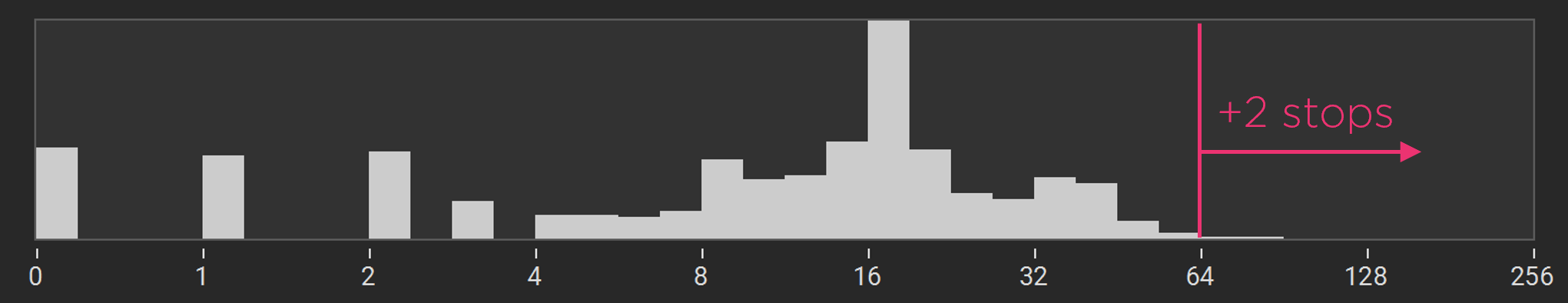
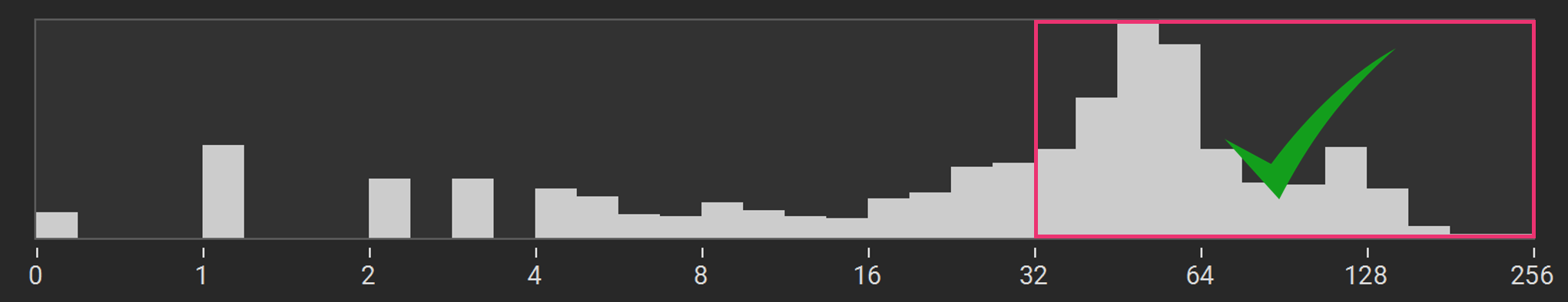
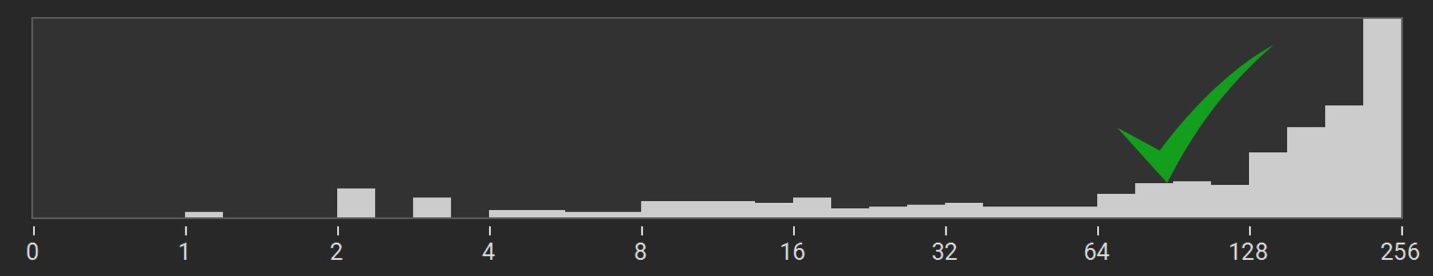
Keep adding acquisitions until almost all pixels are on the right-hand side of the logarithmic histogram, as shown in the image below.
Enjoy the HDR
Enable all acquisitions and capture an HDR to confirm you have covered the increased dynamic range.
Pro tip: further improving noise at the expense of time
If the time budget allows it, duplicate acquisitions to perform additional SNR boosting. Grabbing multiple identical acquisitions is the equivalent of performing over-sampling and will, therefore, suppress noise by up to \(\sqrt{N}\), where \(N\) is the number of acquisitions. Duplicating acquisitions is an excellent way of maximizing point cloud quality at the expense of time. Duplicate the acquisitions exposed for the regions that require higher accuracy.
Be aware of your trade-offs
Exposure Variable |
Pros |
Cons |
Exposure Time |
|
|
Aperture |
|
|
Projector Brightness |
|
|
Gain |
|
|
Note
For Zivid One+, changing Aperture is faster than changing Exposure Time. For Zivid One+, changing Aperture is faster than changing Exposure Time.
Further reading
After the acquisitions have been exposed right it is time to adjust the filters as described in Adjusting Filters