Downsampling

Introduction

This article describes how to correctly downsample a Zivid point cloud. If you are interested in the implementation, check out our downsampling code samples in C++, C#, Python, and MATLAB.

Note

From Zivid SDK v2.1.0 downsampling is implemented in the API.

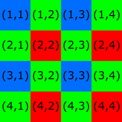
To downsample a point cloud, one might decide to keep every second, third, fourth, etc. pixel from the initial, organized point cloud, discarding all other pixels. However, when it comes to a Zivid camera, this is not the best solution. The reason is that our camera sensor has a Bayer filter mosaic. The grid pattern of the Bayer filter mosaic for a 4 x 4 image is shown in the figure below. Each pixel on the camera image corresponds to one color filter on the mosaic. The numbers in the grid pattern represent image coordinates. Note that some image coordinate systems, such as the one in our API, start with (0,0).

Consider a downsampling algorithm that keeps every other pixel. All kept pixels would correspond to the same color filter for all four possible options:

• (1,1) (1,3) (3,1) (3,3) → Blue

• (2,1) (2,3) (4,1) (4,3) → Green

• (1,2) (1,4) (3,2) (3,4) → Green

• (2,2) (2,4) (4,2) (4,4) → Red

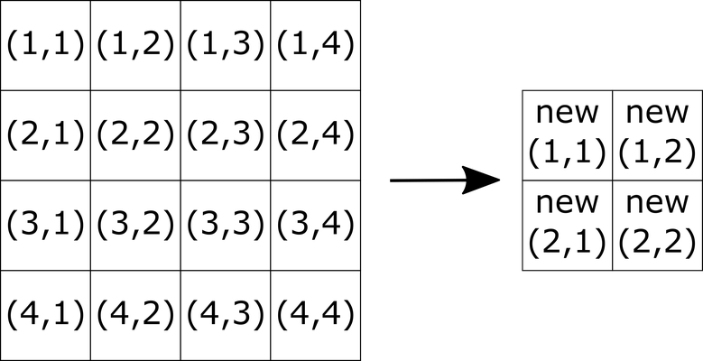
To preserve the quality of data, one should consider all pixels while downsampling a point cloud. In addition, every pixel of the downsampled image should be obtained based on a procedure performed on an even pixel grid (2x2, 4x4, 6x6, etc.) of the original image. A recommended procedure for downsampling a Zivid point cloud is described as follows. It is assumed that the goal is to half the point cloud in size by reducing the image from e.g. 4x4 to 2x2.

Downsampling RGB values (2D image)

Each pixel value of the new image should be calculated by the average over every 2x2 pixel grid of the initial image. This should be done for each channel R, G and B. Here is an example to calculate the new R:

\[\begin{split}\begin{align} R_{new}(1,1) = \frac{R(1,1)+R(1,2)+R(2,1)+R(2,2)}{4}\\ R_{new}(1,2) = \frac{R(1,3)+R(1,4)+R(2,3)+R(2,4)}{4}\\ R_{new}(2,1) = \frac{R(3,1)+R(3,2)+R(4,1)+R(4,2)}{4}\\ R_{new}(2,2) = \frac{R(3,3)+R(3,4)+R(4,3)+R(4,4)}{4} \end{align}\end{split}\]

The same should be done for G and B values.

The same procedure that is used to calculate the R, G, B values can be utilized to calculate the X, Y, Z values of the new downsampled point cloud. When calculating the X, Y, Z values it is also necessary to handle the NaN values in the point cloud. The previous method is therefore not the optimal solution, and a better approach is described below.

Downsampling XYZ values (point cloud)

X, Y, Z pixel values of the new image should be calculated by taking every 2x2 pixel grid of the initial image. Instead of a normal average, an SNR-weighted average value should be used for each coordinate. To brush up on how Zivid uses SNR check out our SNR page.

There are cases where the X, Y, Z coordinates of any pixel may have a NaN value, but the SNR for that pixel will not be NaN. We can handle this by doing a basic check to see if any pixel has a NaN value for one of its coordinates. Check if any pixel has a NaN value for one of the X, Y, Z coordinates. If it does, then replace the SNR value for that pixel with zero. This can be done by selecting the pixels whose e.g. Z coordinates are NaNs and setting their SNR value to zero:

\[SNR(isNAN(Z)) = 0\]

where \(isNAN()\) is a logical masking function that selects only the pixels whose input coordinates are NaNs.

The next step is calculating the sum of SNR values for every 2x2 pixel grid:

\[C_{sum}=SNR(1,1) + SNR(1,2) + SNR(2,1) + SNR(2,2)\]

After this, calculate the weight for each pixel of the initial image:

\[\begin{split}\begin{align} W(1,1) = \frac{SNR(1,1)}{C_{sum}}\\ W(1,2) = \frac{SNR(1,2)}{C_{sum}}\\ W(2,1) = \frac{SNR(2,1)}{C_{sum}}\\ W(2,2) = \frac{SNR(2,2)}{C_{sum}} \end{align}\end{split}\]

To avoid having to deal with \(NaN \cdot 0 = NaN\) instead of \(NaN \cdot 0 = 0\) it is advisable to do the following:

\[\begin{split}\begin{align} & W(isNaN(W)) = 0 \\\\ & X(isNaN(X)) = 0 \\\\ & Y(isNaN(Y)) = 0 \\\\ & Z(isNaN(Z)) = 0 \end{align}\end{split}\]

Finally, the X, Y, Z coordinate values can be calculated. Here is an example for calculating the new X:

\[X_{new}(1,1) = X(1,1) \cdot W(1,1) + X(1,2) \cdot W(1,2) + X(2,1) \cdot W(2,1) + X(2,2) \cdot W(2,2)\]

The same should be done for Y and Z values.

Note that in the sample code, while the underlying concept is the same, the order of operation is slightly different than the above:

\[X_{new}(1,1) = \frac{X(1,1) \cdot SNR(1,1) + X(1,2) \cdot SNR(1,2) + X(2,1) \cdot SNR(2,1) + X(2,2) \cdot SNR(2,2)}{C_{sum}}\]